APSG tutorial - Part 6

Various tricks

The apsg_conf dictionary allows to modify APSG settings.

import numpy as np
from apsg import *
apsg_conf['figsize'] = (9, 7)

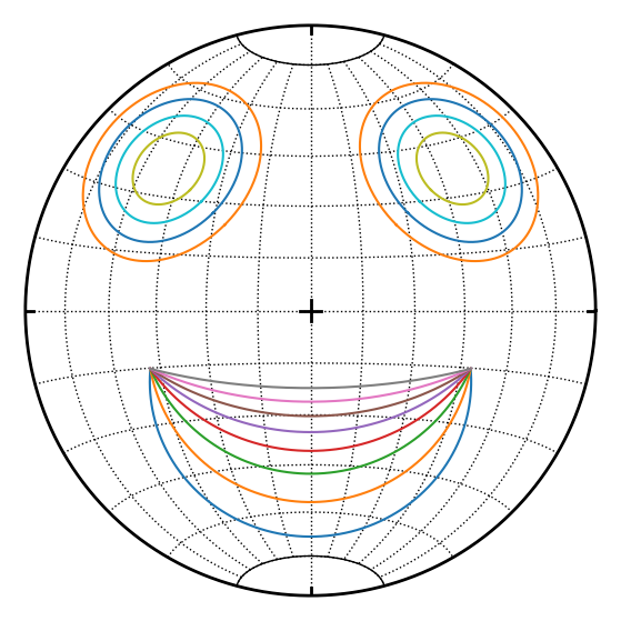
Some fun with cones…

l1 = lin(110, 40)
l2 = lin(250, 40)
m = l1.slerp(l2, 0.5)
p = lin(l1.cross(l2))

s = StereoNet()

for t in np.linspace(0, 1, 8):
    D = defgrad.from_vectors_axis(l1, l2, m.slerp(p, t))
    a, ang = D.axisangle()
    s.cone(cone(a, l1, ang))

for a in np.linspace(10,25,4):
    s.cone(cone(lin(315, 30), a), cone(lin(45, 30), a))

s.show()

Some tricks

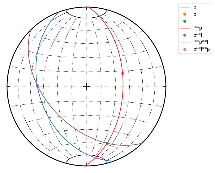
Double cross products are allowed but not easy to understand.

For example p**l**p is interpreted as p**(l**p): a) l**p is plane defined by l and p normal b) intersection of this plane and p is calculated

p = fol(250,40)
l = lin(160,25)
s = StereoNet()
s.great_circle(p, label='p')
s.pole(p, label='p')
s.line(l, label='l')
s.great_circle(l**p, label='l**p')
s.line(p**l, label='p**l')
s.great_circle(l**p**l, label='l**p**l')
s.line(p**l**p, label='p**l**p')
s.show()

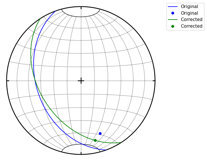
Pair class could be used to correct measurements of planar linear features which should spatialy overlap

pl = pair(250, 40, 160, 25)
pl.misfit

18.889520432245405

s = StereoNet()
s.great_circle(fol(250, 40), color='b', label='Original')
s.line(lin(160, 25), color='b', label='Original')
s.great_circle(pl.fol, color='g', label='Corrected')
s.line(pl.lin, color='g', label='Corrected')
s.show()

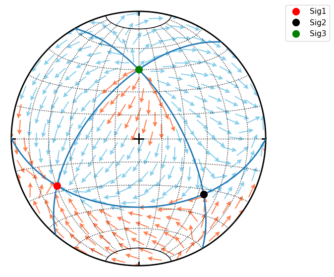
StereoNet has method arrow to draw arrow. Here is example of Hoeppner plot for variable fault orientation within given stress field

R = defgrad.from_pair(pair(180, 45, 240, 27))
S = stress([[-8, 0, 0],[0, -5, 0],[0, 0, -1]]).transform(R)
d = vecset.uniform_gss(n=600)
d = d[~d.is_upper()]
s = StereoNet()
s.great_circle(*S.eigenfols, lw=2)
s.line(S.sigma1dir, ms=10, color='red', label='Sig1')
s.line(S.sigma2dir, ms=10, color='k', label='Sig2')
s.line(S.sigma3dir, ms=10, color='green', label='Sig3')
for n in d:
    f = S.fault(n)
    if f.sense == 1:
        s.arrow(f.fvec, f.lvec, sense=f.sense, color='coral')
    else:
        s.arrow(f.fvec, f.lvec, sense=f.sense, color='skyblue')
s.show()

ClusterSet class

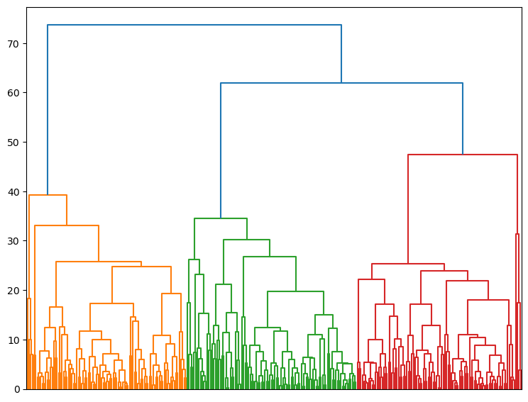
ClusterSet class provide access to scipy hierarchical clustering. Distance matrix is calculated as mutual angles of features within FeatureSet keeping axial and/or vectorial nature in mind. ClusterSet.elbow() method allows to explore explained variance versus number of clusters relation. Actual cluster is done by ClusterSet.cluster() method, using distance or maxclust criterion. Using of ClusterSet is explained in following example. We generate some data and plot dendrogram:

g1 = linset.random_fisher(position=lin(45,30))
g2 = linset.random_fisher(position=lin(320,56))
g3 = linset.random_fisher(position=lin(150,40))
g = g1 + g2 + g3
cl = cluster(g)
cl.dendrogram(no_labels=True)

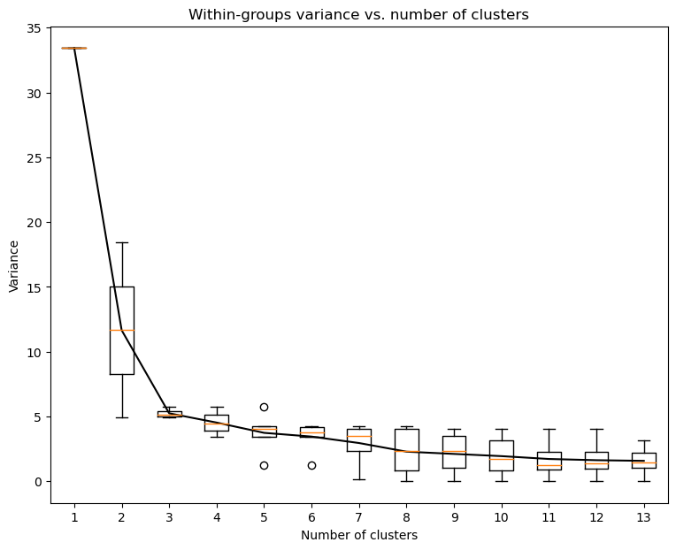
Now we can explore evolution of within-groups variance versus number of clusters on Elbow plot (Note change in slope for three clusters)

cl.elbow()

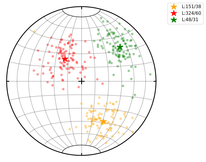
Finally we can do clustering with chosen number of clusters and plot them

cl.cluster(maxclust=3)
cl.R.data  # Restored centres of clusters

(L:151/38, L:324/60, L:48/31)

s = StereoNet()
for gid, color in zip(range(3), ['orange', 'red', 'green']):
    s.line(cl.groups[gid], color=color, alpha=0.4, mec='none')
    s.line(cl.R[gid], ms=16, color=color, marker='*', label=True)
s.show()