APSG tutorial - Part 3

[1]:

from apsg import *

StereoNet class

StereoNet allows to visualize fetaures on stereographic projection. Both equal-area Schmidt (default) and equal-angle Wulff projections are supported.

[2]:

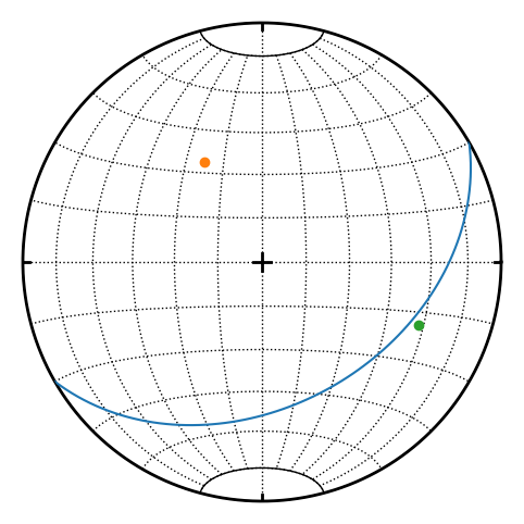
s = StereoNet()
s.great_circle(fol(150, 40))
s.pole(fol(150, 40))
s.line(lin(112, 30))
s.show()

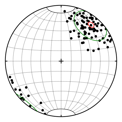
../_images/notebooks_03_apsg_stereonet_3_0.png

A small circles (or cones) could be plotted as well

[3]:

s = StereoNet()
l = linset.random_fisher(position=lin(40, 15), kappa=15)
s.line(l, color='k')
s.cone(l.fisher_cone_a95(), color='r')  # confidence cone on resultant
s.cone(l.fisher_cone_csd(), color='g')  # confidence cone on 63% of data
s.show()

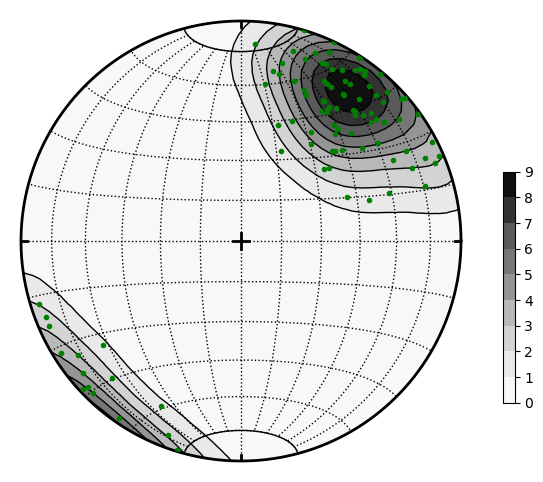
../_images/notebooks_03_apsg_stereonet_5_0.png

For density contouring a contour method is available

[4]:

s = StereoNet()
s.contour(l, levels=8, colorbar=True)
s.line(l, color='g', marker='.')
s.show()

../_images/notebooks_03_apsg_stereonet_7_0.png

APSG also provides pairset and faultset classes to store pair or fault datasets. It can be inicialized by passing list of pair or fault objects as argument or use class methods from_array or from_csv

[5]:

p = pairset([pair(120, 30, 165, 20),
             pair(215, 60, 280,35),
             pair(324, 70, 35, 40)])
p.misfit

[5]:

array([0.00000000e+00, 1.42108547e-14, 0.00000000e+00])

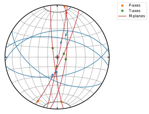
StereoNet has two special methods to visualize fault data. Method fault produce classical Angelier plot

[6]:

f = faultset([fault(170, 60, 182, 59, -1),
              fault(210, 55, 195, 53, -1),
              fault(10, 60, 15, 59, -1),
              fault(355, 48, 22, 45, -1)])
s = StereoNet()
s.fault(f)
s.line(f.p, label='P-axes')
s.line(f.t, label='T-axes')
s.great_circle(f.m, label='M-planes')
s.show()

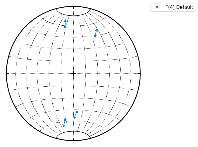
../_images/notebooks_03_apsg_stereonet_11_0.png

hoeppner method produce Hoeppner diagram and must be invoked from StereoNet instance

[7]:

s = StereoNet()
s.hoeppner(f, label=repr(f))
s.show()

../_images/notebooks_03_apsg_stereonet_13_0.png

StereoGrid class

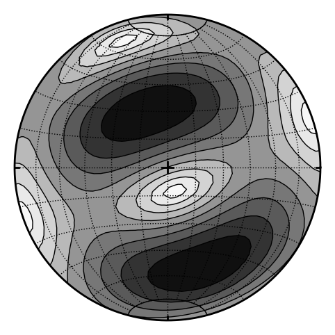
StereoGrid class allows to visualize any scalar field on StereoNet. It is used for plotting contour diagrams, but it exposes apply_func method to calculate scalar field by any user-defined function. Function must accept three element numpy.array as first argument passed from grid points of StereoGrid.

Following example defines function to calculate resolved shear stress on plane from given stress tensor. StereoGrid accesses via .grid property is used to calculate this value over all directions and finally values are plotted by StereoNet

[8]:

S = stress([[-10, 2, -3],[2, -5, 1], [-3, 1, 2]])
s = StereoNet()
s.grid.apply_func(S.shear_stress)
s.contour(levels=10)
s.show()

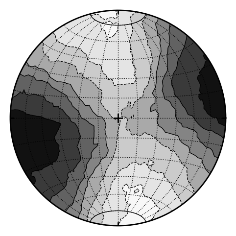
../_images/notebooks_03_apsg_stereonet_16_0.png

The StereoGrid provide also amgmech (Angelier dihedra) method for paleostress analysis. Results are stored in StereoGrid. Default behavior is to calculate counts (positive in extension, negative in compression)

[9]:

f = faultset.from_csv('mele.csv')
s = StereoNet()
s.grid.angmech(f)
s.contour()
s.show()

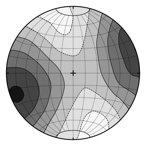
../_images/notebooks_03_apsg_stereonet_18_0.png

Setting method to probability, maximum likelihood estimate is calculated.

[10]:

f = faultset.from_csv('mele.csv')
s = StereoNet()
s.grid.angmech(f, method='probability')
s.contour()
s.show()

../_images/notebooks_03_apsg_stereonet_20_0.png

[11]:

s.grid

[11]:

StereoGrid EqualAreaProj 3000 points.
Maximum: 48.3587 at L:250/11
Minimum: -36.1316 at L:158/14

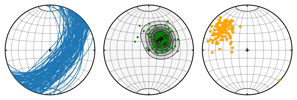
Multiple stereonets in figure

[12]:

import matplotlib.pyplot as plt

fig = plt.figure(constrained_layout=True, figsize=(10, 4))
subfigs = fig.subfigures(1, 3)

f = folset.random_fisher(position=fol(130, 60))
l = linset.random_fisher(position=fol(230, 30))
# panel 1
s1 = StereoNet()
s1.great_circle(f)
# panel 2
s2 = StereoNet()
s2.contour(l)
s2.line(l, ms=4, color='green')
# panel 3
s3 = StereoNet()
s3.pole(f, color='orange')
# render2fig
s1.render2fig(subfigs[0])
s2.render2fig(subfigs[1])
s3.render2fig(subfigs[2])
plt.show()

../_images/notebooks_03_apsg_stereonet_23_0.png

[ ]: